Next.Buy: recommend your user's next purchase
Insight data science project

During my stay at Insight Data Science, I worked on a consulting project for a company who provides retailers with the opportunity to communicate with their customers after the sale is made. This way, retailers can make personalized offers to their customers. My goal as consultant was to offer some insight on the kind of offers that could be made, by predicting the next purchase a given user would be the most likely to make, based on her/his purchase histories, demographic specificities and a given retailer. A good way to do this is by generating a recommendation model which presents a ranked list of objects (e.g. products) given an input object (another product) or a user. I used a two-step strategy to tackle the high sparsity of my data.
Next.Buy Demo
Next.Buy: the project
The company’s MySQL database is located on a remote server. It contains information about more than 260M products, purchased by 9M users, in 6000 stores from 40 retailers across the USA and Canada.

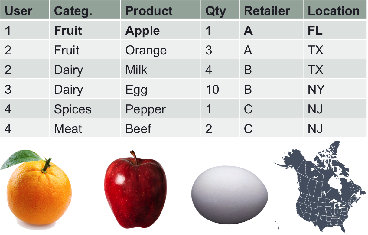
The Non-Disclosure Agreement (NDA) associated to this project prohibits me to name retailers and any other features that could identify them, so I will refer to them with different names, such as retailer A, B, C. Each product is characterized by several features, including the following: a description (name, e.g. “banana”), a category (e.g. “fruit”), the quantity bought for each purchase, the location of the purchase (store and store address), and the retailer name.
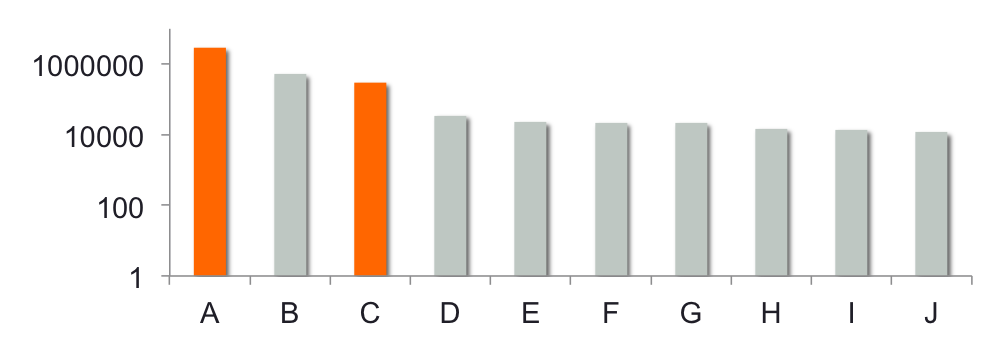
The fact that the server is distant causes the SQL queries to be extremely slow, which in turn means that I can only pull a limited amount of users and their purchase history. Since the deliverable calls for a model that is both demographic and merchant specific, I start by characterizing “who buys where”. The graph below (Fig. 1) represents the number of users for the top 10 biggest retailers. The 3 first retailers, A, B and C totalize most of the users (>94%).
Figure 1. Number of users per retailer.
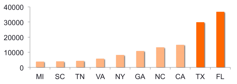
Another interesting data to look at is where the most purchases are made, using the store’s address (state) as a proxy for the user’s location. About a third of the purchases for retailer A are made in Florida and Texas (Fig. 2).
Figure 2. Number of purchases made per state for retailer
Collaborative filtering
I will this focus the model on these particular population subsets: FL and TX, retailers A and C.
This scenario calls for a model that is optimal for characterizing the large number of users/items in the data set (9M/260M), but that can still be estimated for the limited amount of users (between 5000 and 10000) and products (2000 for merchant C) available in the population subsets. Collaborative filtering appears to be a suitable option, as it assesses users or item’s similarity to predict user’s preference. For example, if two users 1 and 2 tend to watch and like similar kinds of movies, the likelihood that user 1 will like a movie that user 2 likes too is high. The liking is usually assessed by a rating, for example from 1 (very bad movie) to 5 (very good movie).
The date is organized in a user - item matrix with N rows x M columns, where N are users and M items (in Machine learning, N are called ‘samples’ and M,’features’). In this example, the item is the product or the category that is being recommended. The matrix is populated with user-item pairs, corresponding to an event (e.g. rating when a given user rated a given item, or an empty entry when a given user did not rate the given item, often modelized with a 0). Sparsity corresponds to the proportion of user-item pairs that actually have data.
In this example, two adaptations are made:
-
Since there is no information about how the customers like their purchase (no ratings), the quantity of items purchased is taken as a proxy for users’s preference to populate the user - item matrix, with a 0 entry when no purchase is made (Fig. 3 and 4).
-
The user - product matrix is too sparse (less than 0.1%) to come up with a direct product recommendation. Therefore the category information provided in the dataset is used as an intermediate recommendation step to reduce dimensionality. Again, the NDA prevents me to reveal true information about the products so I replace actual categories designation with grocery categories and product names with grocery items. Since the number of categories in retailer B is limited, the model is estimated only for retailers A and C in this example.
Figure 3. Number of purchases made per category for retailer C.
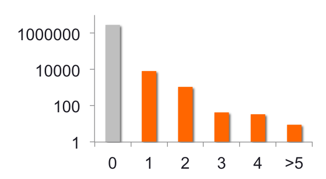
Figure 4. Distribution of purchases made for category “fruits”, retailer C as a function of the quantity of items bought
A two-step recommender system
train and test phase
Leave k out: a split percentage is chosen (e.g., 80% train, 20% test) and the test percentage is selected randomly from the user-item pairs with non-zero entries.
Category recommendation
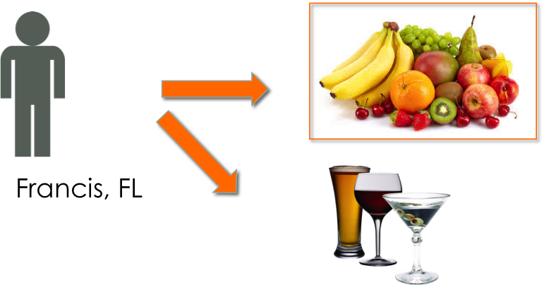
I train a model per each location (state: FL and TX) and retailer (merchant A and C) The way the model works is the following: Francis, a user from FL, will be recommended with various categories according to his purchase history and his similarity with other users from FL (User-based recommendation). These categories will be ranked from most likely (fruits) to least likely (drinks), as function of similarity scores. Here, Francis most recommended category is “Fruits”.
The User-based recommendation system used in this example considers similarities between user consumption histories and item similarities. Cosine Similarity, measured as the cosine of the angle between the users’ or two item’ vectors, assesses the user-user or the item-item distance.
Product recommendation
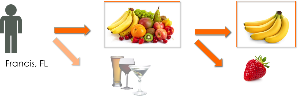
Once a given category has been recommended, the user will be recommended with products within it. In this case, Francis is recommended with “banana”.
Repurchase score & recommendation
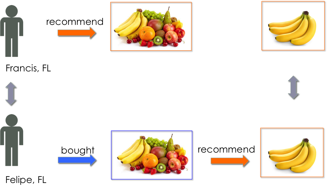
In this particular model, to avoid recommending something that was already purchased, items (categories or products) that were already bought by a given user are assigned with a similarity score of zero, so thay they do not appear in top of the recommendation. Therefore, there is a high likelihood that the most recommended category for Francis is one that he did not purchase into. This means that we can very well have no data for Francis at the product level within this category. In other terms, how could we recommend a given fruit (banana, apple, strawberry…), if Francis did not buy any fruits at all?
The solution is to APPROXIMATE Francis’s behavior by that of his most similar user within Florida, Felipe, that bought within the “Fruits” category, and look at Felipe’s 1st recommendation at the product level.
It is important to note that the user behavior will vary greatly as function of the kind of items sold by a retailer. It is sometimes preferable for the model to keep recommending items that were already bought, if for example, we are designing a recommendation algorithm for a grocery store, because the likelihood to purchase the same items again and again is high (e.g. milk, bread). This is known as a high repurchase score. This kind of recommendation might be useful if a discount offer wants to be made for a given customer on his/her most often purchased products. On the other hand, if the aim of the algorithm is to recommend a new item, then some serendipity should be taken into account in the system to avoid recommending milk all the time (e.g. by taking the k-th recommendation out of the n possibilities, instead of the first)
On the other hand, other retailers (e.g. furniture store) will sell items that are not bought frequently, i.e. with a low repurchase score (e.g. bed, sofa). In this case, the model could be adapted by suppressing the already bought items from the recommendation.
Finally, in the case of a a retailer that sells both high and low repurchase score items, a possible solution would be to weigh the recommendation of these items according to their repurchase score.
The repurchase score can be intuitively understood as a combination of how popular an item is (number of times an item was purchased) and whether these items were purchased over several days. It can be estimated by assessing the frequency with which a given item was rated / bought by a given user. This implies having access to a long history of purchases (over a year for example), which unfortunately was impossible with the small subsample studied here.
Insights on local shopping behavior
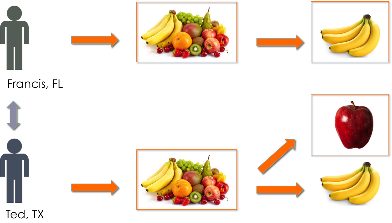
The recommender models described here are specic to each retailer and location, offering the possibility to compare user behaviors geographically. If we examine the recommendations made for Ted, Francis’s most similar user in TX, we can see that Ted is recommended with the “Fruit” category’, but instead of “banana”, he is recommended with “apple”.
With sufficient computational power, this algorithm could be run on all possible users from all locations. By cumulating the comparisons accross states, the model could eventually provide quantitative insight on local shopping behavior, and thus infer suggestions to retailers on how to adjust their product offer according to location.
Validation metrics
Distinguishing between good and bad recommendations is part of what we want to achieve with recommender systems. A binarization threshold determines which data is ‘good’ (or labeled as 1) or bad (0) when dealing with non-binary data (such as ratings or purchased quantities in our case). For both category and product recommendation, this threshold is set to 1.1 as the distribution of items suggests a vast majority of unique purchases (see Fig. 4).
The classification metrics (ranging from 0 to 1) used in other machine learning algorithms (e.g. binary classification) are thus suitable here. The Receiver Operator Characteristic (ROC) curve, a toll used in classification, plots the True Positive Rate against the False Positive rate and this enables to summarize the performance of the model. It can be summarized by its integral, or Area Under the Curve (AUC-ROC). Recall represents the ability of the classifier to fun all positive samples, while precision represents the ability of the classifier not label as positive a sample that is negative.
Since we are producing a ranking of the best possible items to recommend for each user, a useful rank-based metric is the Normalized Discounted Cumulative Gain (NDCG). NDCG also ranges from 0 to 1, and emphasizes that items with high relevance should be placed early in the ranked list, without binarizing the data.
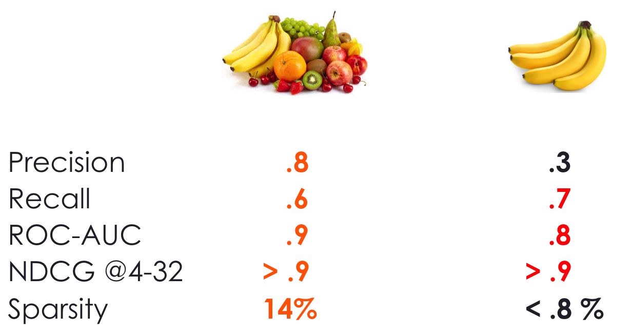
Figure 5 shows the validation metrics for boths steps of the recommender system. On the left (category choice), both classification metrics and ranking metrics suggest a good prediction and accurate ranking of relevant items. On the right (product choice), the metrics are generally good with the exception of precision. This is possibly due to the small sample of users (5000) vs large amount of products (400), resulting in a very sparse user-item matrix (less than 0.1%). The results can be optimized if the model is run on more users.
Figure 5
Improvements
- Use Pearson coefficients / euclidean distances in lieu of cosine similarity
- Different clustering of products than by category, e.g. using Principal Components Analysis or Singular Value Decomposition
- Weighing the recommendations by the repurchase score (or a probability for a given user to buy a given category / product again).
For more on recommender systems